
This notebook demonstrates how to obtain and pre-process satellite data from from NASA LP DAAC - Land Processes Distributed Active Archive Center. I will show how to process LP DAAC datasets into common and easy to use formats for downstream geospatial data processing and scientific analysis. Here we will obtain the Terra and Aqua combined Burned Area data product MCD64A1. This data is a monthly, global gridded 500 meter (m) product containing per-pixel burned-area and quality information.
1
2
3
4
5
6
7
8
9
10
import os
import re
import time
from bs4 import BeautifulSoup
import numpy as np
import rasterio as rio
from osgeo import gdal
import requests
import dotenv
dotenv.load_dotenv(dotenv.find_dotenv())
Obtaining data from LP DAAC - Land Processes Distributed Active Archive Center
The LP DAAC data is organised into:
- folder directories per year-month
- HDF files per sinusoidal grid unit
To limit the number of requests we will obtain data for 1 month over the USA.
1
2
3
4
5
6
7
8
9
10
11
12
13
# params fo LP DAAC
# you will require an EarthData login
host = fr'https://e4ftl01.cr.usgs.gov/MOTA/MCD64A1.061'
login = os.getenv('user')
password = os.getenv('pwd')

# list folders
r = requests.get(host, verify=True, stream=True,auth=(login,password))
soup = BeautifulSoup(r.text, "html.parser")
folders = list()
for link in soup.findAll('a', attrs={'href': re.compile("\d{4}.\d{2}.\d{2}/")}):
    folders.append(link.get('href'))
print(f"{len(folders)} folders found")
1
130 folders found
1
2
3
4
5
6
7
8
9
# list files in folder
for f in folders[:1]:
    file_list = list()
    folder_url = f"{host}/{f}"
    r = requests.get(folder_url, verify=True, stream=True,auth=(login,password))
    soup = BeautifulSoup(r.text, "html.parser")
    for link in soup.findAll('a', attrs={'href': re.compile(".hdf$")}):
        file_list.append(link.get('href'))
print(f"{len(file_list)} files found in folder n")
1
268 files found in folder n
This MODIS data product is delivered in the sinusoidal grid projection. We can apply regex to filter the query to just those tiles over the USA. Note how this projection warps the USA and other regions - we will need to account for this later.
1
2
3
4
5
6
7
8
9
10
11
12
13
# USA tiles only
# use modis grid to slice only continents / areas of interest
# https://modis-land.gsfc.nasa.gov/MODLAND_grid.html
hreg = re.compile("h0[8-9]|h1[0-4]")
vreg = re.compile("v0[2-7]")
usa_files = list()
for fl in file_list:
    h = hreg.search(fl)
    if h:
        v = vreg.search(h.string)
        if v:
            usa_files.append(v.string)
print(f"{len(usa_files)} USA tiles found")
1
34 USA tiles found
1
2
3
4
5
6
7
8
9
10
11
12
13
14
15
16
17
18
# download file from folder
# implement 25 file timeout to avoid rate limit

exceptions = list()
for f in folders[:1]:
    for e,fl in enumerate(usa_files[:]):
        if (e+1) % 10 == 0:
            print('sleep')
            time.sleep(5)
        else:
            print(fl,e+1)
            try:
                file_url = f"{host}/{f}/{fl}"
                r = requests.get(file_url, verify=True, stream=True,auth=(login,password))
                open(f'./data/raw/{fl}',"wb").write(r.content)
            except Exception as error:
                print(error)
                exceptions.append(fl)
1
2
MCD64A1.A2000306.h08v03.061.2021085164213.hdf 1
MCD64A1.A2000306.h08v04.061.2021085165152.hdf 2
MODIS HDF files and CRS
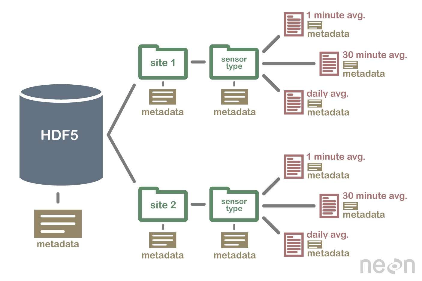
HDF files are self describing - this means that all elements (the file itself, groups and datasets) can have associated meta-data that describes the information contained within the element. You can read more about HDF files in my previous post on MODIS.
The MODIS land products are produced at 4 resolutions (250m, 500m, 1km, and 0.05 degree), and in 3 projections (Sinusoidal, Lambert Azimuthal Equal-Area, and Geographic). The simple Geographic lat/lon projection is only used for the coarsest resolution grid, produced at 0.05 km (~ 5.5 km), which is referred to as the Climate Modeling Grid (CMG). In order to maintain reasonable file sizes for the other higher resolution MODIS land data products, each projection is divided up into a tiled grid.
Geospatial data products have a coordinate reference system (CRS). The CRS refers to the way in which spatial data are represented over the earth’s surface. Most people will be familiar with the WGS 84 (EPSG:4326) CRS as this is widely used in global mapping products like Google or Apple maps. There are many CRS that provide varying degrees of accuracy across the globe, CRS are chosen to suit the needs of the data analysis or application. See more on CRS here
To work more efficiently with these data we will i) translate them to geotiff format which is essentially an array with spatial information, and ii) reproject the data to a common CRS. There are a number of methods and tools to peform these tasks including:
- MODIS GUI tools distributed wiht the data
- Programming tools in Python and R
We want a programmatic method when working with large data and repetitive geospatial datasets. Below are two methods to convert MODIS data using python packages fro GDAL and Rasterio.
GDAL Warp
GDAL is a command line executable. The cmd to run on the terminal is:
1
!gdalwarp -of GTiff -t_srs "EPSG:4326" HDF4_EOS:EOS_GRID:".\MCD64A1.A2000306.h08v04.061.2021085165152.hdf":MOD_Grid_Monthly_500m_DB_BA:"Burn Date" test.tif
and the python binding is as follows:
1
2
3
4
5
6
7
8
9
10
11
12
for fl in usa_files[:]:
    in_file = f"./data/raw/{fl}"
    out_file = f"./data/transformed/{fl.replace('.hdf','.tif')}"

    # open dataset
    dataset = gdal.Open(in_file,gdal.GA_ReadOnly)
    subdataset =  gdal.Open(dataset.GetSubDatasets()[0][0], gdal.GA_ReadOnly)

    # gdalwarp
    kwargs = {'format': 'GTiff', 'dstSRS': 'EPSG:4326'}
    ds = gdal.Warp(destNameOrDestDS=out_file,srcDSOrSrcDSTab=subdataset, **kwargs)
    del ds
Loading the output from gdal into QGIS (or any visualisation tool) we see the transformed data in relation to WGS84 global shorelines, and we can see the warp (curve) effect at the tile boundaries. This warp is created from translating the MODIS tiles from native Sinusoidal tiles to WGS84 Mercator grid. But you can see how the blue (water), green (no burn) MODIS shaded area’s lie within the shoreline data confirming that the translation was successful. There are few burn areas (red) visible in this image as we are zoomed out in order to see the translation.

Rasterio
Rasterio is a dedicated python package for geospatial data and analytics. The library provides more granular access and options to low level functions, at the expense of brevity. If you need to perform some bespoke transformations and operations, or want to optimise your pipeline for larger datasets, rasterio is a good option.
1
2
3
4
5
6
7
8
9
10
11
12
13
14
15
16
17
18
19
20
21
22
23
24
25
26
27
28
29
30
31
32
33
34
35
36
37
38
39
40
41
42
43
44
45
46
47
48
49
50
51
52
53
54
55
56
# from rasterio.warp import calculate_default_transform, reproject, Resampling
# for fl in [fl for fl in usa_files if fl == 'MCD64A1.A2000306.h08v04.061.2021085165152.hdf']:

#     file_name = f'./data/{fl}'

#     all_bands = []

#     with rio.open(file_name) as dataset:
#         # capture meta and CRS data
#         hdf4_meta = dataset.meta
#         crs = dataset.read_crs()

#         # iterate data layers and select using name
#         for layer_name in dataset.subdatasets[:1]:
#             #print(layer_name)
#             with rio.open(layer_name) as subdataset:
#                 bounds = subdataset.bounds
#                 modis_meta = subdataset.profile
#                 all_bands.append(subdataset.read(1))

#         # prep metadata object
#         output_meta = modis_meta.copy()
#         output_meta['driver'] = 'GTiff'
#         output_meta['count'] = 1 # all_bands[0].shape[0]

#         with rio.open(out_path, "w", **kwargs) as dest:
#             dest.write(all_bands[0],indexes=1)

#         # reproject to 4326
#         dst_crs = "EPSG:4326"
#         transform, width, height = calculate_default_transform(output_meta.data['crs'],
#                                                                dst_crs,
#                                                                output_meta.data['width'],
#                                                                output_meta.data['height'],
#                                                                *bounds,
#                                                                dst_width=output_meta.data['width'],
#                                                                dst_height=output_meta.data['height'],)
#         kwargs = modis_meta.copy()
#         kwargs.update({'crs': dst_crs,
#                        'transform': transform,
#                        'width': width,
#                        'height': height})

#         # reproject and write to file e as a geotiff
#         out_path = f'{fl}.tif'
#         ino = all_bands[0]
#         ooo = all_bands[0].copy()
#         with rio.open(out_path, "w", **kwargs) as dest:
#             reproject(source=ino,
#                       destination=ooo,
#                       src_transform=modis_meta.data['transform'],
#                       src_crs=modis_meta.data['crs'],
#                       dst_transform=transform,
#                       dst_crs=dst_crs,
#                       resampling=Resampling.nearest)
References
- global shorlines
- python Gdal
- read HDF in gdal
- gdal Warp documentation
- how to use gdal Warp()
- https://developers.google.com/earth-engine/datasets/catalog/JRC_GWIS_GlobFire_v2_FinalPerimeters#description
- https://www.nature.com/articles/s41597-019-0312-2
- https://lpdaac.usgs.gov/products/mcd64a1v061/
- https://git.earthdata.nasa.gov/projects/LPDUR
- https://hdfeos.org/forums/showthread.php?t=496
- https://git.earthdata.nasa.gov/projects/LPDUR/repos/2020-agc-workshop/browse
- https://modis.gsfc.nasa.gov/tools/
- https://modis-land.gsfc.nasa.gov/MODLAND_grid.html
- Converting MODIS HDFs with sinusoidal projections to ArcGIS raster format
- Welcome to GDAL notes’s documentation!
- Official MODIS authentication Python and R scripts
1
2