

The Moderate Resolution Imaging Spectroradiometer (MODIS) is an imaging sensor built by Santa Barbara Remote Sensing that was launched into Earth orbit by NASA in 1999 on board the Terra (EOS AM) satellite, and in 2002 on board the Aqua (EOS PM) satellite. The instruments capture data in 36 spectral bands and has a 2,330-km-wide viewing swath, seeing every point on earth every 1-2 days.
Given its wide spectral band, high frequency and temporal coverage MODIS is used in a variety of applications. From measuring atmospheric variables including: cloud cover, the size of cloud droplets in both liquid water and ice particles, aerosols and pollution from natural and man-made sources like industry emissions, dust storms, volcanic eruptions, and forest fires.
This notebook demonstrates how to: download MODIS data; extract meta-data and data from native HDF files; and to transform HDF data to common downstream formats for processing, analysis and plotting.
Download a MODIS tile
1
2
3
4
5
6
tile = 'MCD19A1.A2020246.h08v05.006.2020270073445'
url = fr'https://e4ftl01.cr.usgs.gov/MOTA/MCD19A1.006/2020.09.02/{tile}.hdf'
login = os.getenv('user')
password = os.getenv('pwd')
r = requests.get(url, verify=True, stream=True,auth=(login,password))
open(f'{tile}.hdf',"wb").write(r.content)
Load Data from MODIS HDF

HDF files are self describing - this means that all elements (the file itself, groups and datasets) can have associated meta-data that describes the information contained within the element.
Rasterio is used to iterate through the layers contained in the HDF file. A condition is used to extract the spectral bands 1-7 data.
1
2
3
4
5
6
7
8
9
10
11
12
all_bands = []
with rio.open(f'{tile}.hdf') as dataset:
    # capture meta and CRS data
    hdf4_meta = dataset.meta
    crs = dataset.read_crs()

    # iterate data layers and select using name
    for layer_name in [name for name in dataset.subdatasets if 'grid500m:Sur_refl_500m' in name]:
        print(layer_name)
        with rio.open(layer_name) as subdataset:
            modis_meta = subdataset.profile
            all_bands.append(subdataset.read(1))
1
2
3
4
5
6
7
HDF4_EOS:EOS_GRID:MCD19A1.A2020246.h08v05.006.2020270073445.hdf:grid500m:Sur_refl_500m1
HDF4_EOS:EOS_GRID:MCD19A1.A2020246.h08v05.006.2020270073445.hdf:grid500m:Sur_refl_500m2
HDF4_EOS:EOS_GRID:MCD19A1.A2020246.h08v05.006.2020270073445.hdf:grid500m:Sur_refl_500m3
HDF4_EOS:EOS_GRID:MCD19A1.A2020246.h08v05.006.2020270073445.hdf:grid500m:Sur_refl_500m4
HDF4_EOS:EOS_GRID:MCD19A1.A2020246.h08v05.006.2020270073445.hdf:grid500m:Sur_refl_500m5
HDF4_EOS:EOS_GRID:MCD19A1.A2020246.h08v05.006.2020270073445.hdf:grid500m:Sur_refl_500m6
HDF4_EOS:EOS_GRID:MCD19A1.A2020246.h08v05.006.2020270073445.hdf:grid500m:Sur_refl_500m7
Transform Spectral Bands 1-7
The spectral bands are then stacked to a n-dimension array.
1
2
3
4
# Stack pre-fire reflectance bands
pre_fire_modis = np.stack(all_bands)
print(f'Shape: {pre_fire_modis.shape}')
print(f'Meta: {modis_meta}')
The last layer provides metadata for the layers.
1
2
3
Shape: (7, 2400, 2400)
Meta: {'driver': 'HDF4Image', 'dtype': 'int16', 'nodata': -28672.0, 'width': 2400, 'height': 2400, 'count': 4, 'crs': CRS.from_wkt('PROJCS["unnamed",GEOGCS["Unknown datum based upon the custom spheroid",DATUM["Not specified (based on custom spheroid)",SPHEROID["Custom spheroid",6371007.181,0]],PRIMEM["Greenwich",0],UNIT["degree",0.0174532925199433,AUTHORITY["EPSG","9122"]]],PROJECTION["Sinusoidal"],PARAMETER["longitude_of_center",0],PARAMETER["false_easting",0],PARAMETER["false_northing",0],UNIT["Meter",1],AXIS["Easting",EAST],AXIS["Northing",NORTH]]'), 'transform': Affine(463.31271652791725, 0.0, -11119505.196667,
       0.0, -463.3127165279167, 4447802.078667), 'tiled': False}
1
2
# Mask no data values
pre_fire_modis = ma.masked_where(pre_fire_modis == modis_meta["nodata"], pre_fire_modis)
1
2
3
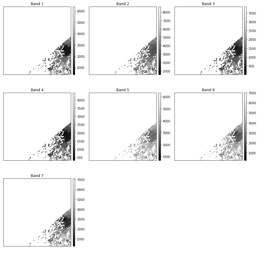
# plot
ep.plot_bands(pre_fire_modis,scale=False,cols=3)
plt.show()
1
2
3
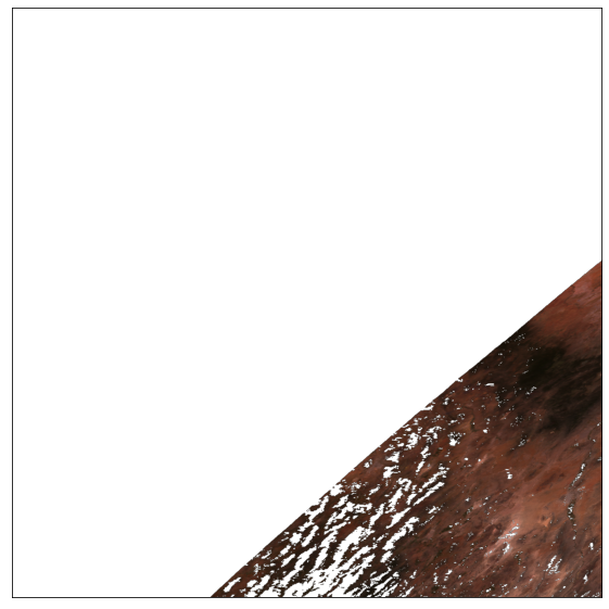
# plot Red, Green and Blue bands
ep.plot_rgb(pre_fire_modis,rgb=[0,3,2]) # RGB bands 1,4,3 (see user guide)
plt.show()
Write to GeoTiff A new meta-data description is created and used to write the stacked array to common GeoTiff format. The key changes are to update the driver variable to ‘GTiff’ and the count variable to the shape of the n-dimension array. In this case count is set to 7 for the seven spectral bands.
1
2
3
4
5
# prep metadata object
output_meta = modis_meta.copy()
output_meta['driver'] = 'GTiff'
output_meta['count'] = pre_fire_modis.shape[0]
output_meta
1
2
{'driver': 'GTiff', 'dtype': 'int16', 'nodata': -28672.0, 'width': 2400, 'height': 2400, 'count': 7, 'crs': CRS.from_wkt('PROJCS["unnamed",GEOGCS["Unknown datum based upon the custom spheroid",DATUM["Not specified (based on custom spheroid)",SPHEROID["Custom spheroid",6371007.181,0]],PRIMEM["Greenwich",0],UNIT["degree",0.0174532925199433,AUTHORITY["EPSG","9122"]]],PROJECTION["Sinusoidal"],PARAMETER["longitude_of_center",0],PARAMETER["false_easting",0],PARAMETER["false_northing",0],UNIT["Meter",1],AXIS["Easting",EAST],AXIS["Northing",NORTH]]'), 'transform': Affine(463.31271652791725, 0.0, -11119505.196667,
       0.0, -463.3127165279167, 4447802.078667), 'tiled': False}
1
2
3
4
out_path = f'{tile}.tif'
# Export file as a geotiff
with rio.open(out_path, "w", **output_meta) as dest:
    dest.write(pre_fire_modis)
Load & Re-project GeoTiff CRS
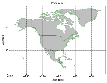
To test that has worked the geotiff is re-loaded and plotted against some country boundaries. Geopandas has a convenient global country dataset for plotting.
1
2
3
4
5
6
7
8
9
10
fig, ax = plt.subplots(figsize=(7,7))
countries = geopandas.read_file(geopandas.datasets.get_path('naturalearth_lowres'))
NA = countries.loc[countries['continent']=='North America']
NA.plot(ax=ax, edgecolor='green',facecolor='grey',alpha=0.5)
ax.set_xticks(np.arange(-180,0,30))
ax.set_yticks(np.arange(0,90,30))
ax.set_xlabel('Longitude')
ax.set_ylabel('Latitude')
ax.grid(True,color='black',lw=0.5,linestyle='--')
ax.set_title(f"EPSG:{NA.crs.to_epsg()}");
However, in order to plot our MODIS Bands1-7 GeoTiff we will need to re-project the data from EPSG:9122 to the same CRS EPSG:4326 as GeoPandas. We can do this using rasterio (see also this guide from Earth Lab at University of Colorado, Boulder).
Altering CRS and re-projection is useful for many geospatial analysis. The OSGEO GDAL “Geospatial Data Abstraction Library” is another great tool for re-projection and QGIS provide a nice background on the topic here
1
2
3
4
5
6
7
8
9
10
11
12
13
14
15
16
17
18
19
20
21
22
23
24
25
26
# Set desitnation CRS
# rio.crs.CRS.from_epsg(4326)
dst_crs = f"EPSG:{NA.crs.to_epsg()}"

# set out path
out_path_rproj = out_path.replace('.tif','-4326.tif')

with rio.open(out_path) as src:
    # get src bounds and transform
    transform, width, height = calculate_default_transform(src.crs, dst_crs, src.width, src.height, *src.bounds)
    kwargs = src.meta.copy()
    kwargs.update({'crs': dst_crs,
                   'transform': transform,
                   'width': width,
                   'height': height})

    # reproject and write to file
    with rio.open(out_path_rproj, 'w', **kwargs) as dst:
        for i in range(1, src.count + 1):
            reproject(source=rio.band(src, i),
                      destination=rio.band(dst, i),
                      src_transform=src.transform,
                      src_crs=src.crs,
                      dst_transform=transform,
                      dst_crs=dst_crs,
                      resampling=Resampling.nearest)
And then plot.
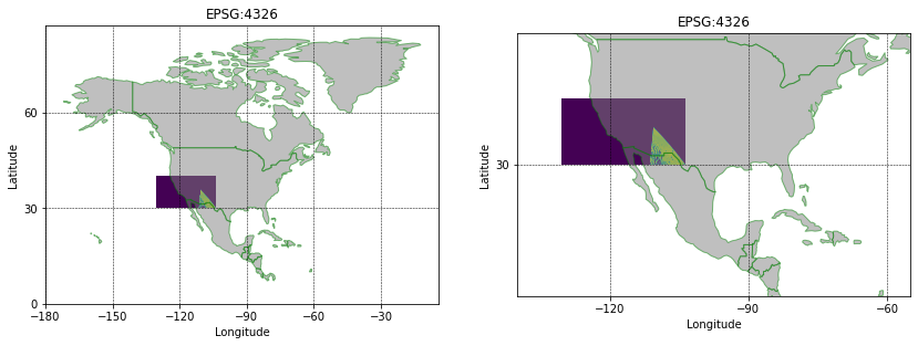
Thanks for reading,