This notebook is a deep dive into General Linear Models (GLM’s) with a focus on the GLM’s used in insurance risk modeling and pricing (Yan, J. 2010).I have used GLM’s before including: a Logistic Regression for landslide geo-hazards (Postance, 2017), for modeling extreme rainfall and developing catastrophe models (Postance, 2017). The motivation for this post is to develop a deeper knowledge of the assumptions and application of the models and methods used by Insurance Actuaries, and to better understand how these compare to machine learning methods.
Case study dataset: motorcylce insurance
The Ohlsson dataset is from a former Swedish insurance company Wasa. The data includes aggregated customer, policy and claims data for 64,548 motorcycle coverages for the period 1994-1998. The data is used extensively in actuarial training and syllabus worldwide Ohlsson, (2010).
Variables include:
- data available here
| dtype | null | nunique | |
|---|---|---|---|
| Age | float64 | 0 | 85 |
| Sex | category | 0 | 2 |
| Geog | category | 0 | 7 |
| EV | category | 0 | 7 |
| VehAge | int64 | 0 | 85 |
| NCD | category | 0 | 7 |
| PYrs | float64 | 0 | 2577 |
| Claims | int64 | 0 | 3 |
| Severity | float64 | 0 | 590 |
| Claim | int64 | 0 | 2 |
| SeverityAvg | float64 | 0 | 590 |
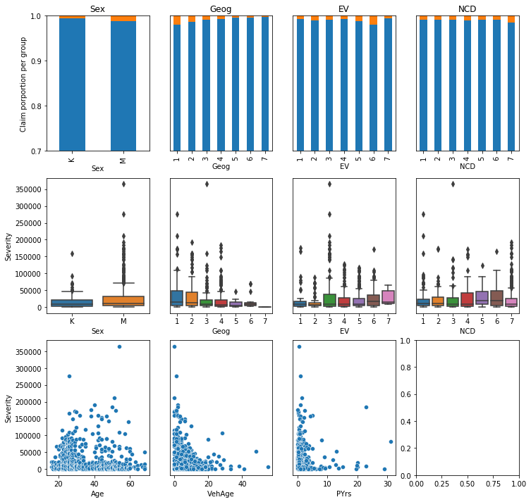
EDA
All data: low number of claims and frequency (1% freq)
| Age | VehAge | PYrs | Claims | Severity | Claim | SeverityAvg | |
|---|---|---|---|---|---|---|---|
| count | 64548.000000 | 64548.000000 | 64548.000000 | 64548.000000 | 64548.000000 | 64548.000000 | 64548.000000 |
| mean | 42.416062 | 12.540063 | 1.010759 | 0.010798 | 264.017785 | 0.010380 | 246.964360 |
| std | 12.980960 | 9.727445 | 1.307356 | 0.107323 | 4694.693604 | 0.101352 | 4198.994975 |
| min | 0.000000 | 0.000000 | 0.002740 | 0.000000 | 0.000000 | 0.000000 | 0.000000 |
| 25% | 31.000000 | 5.000000 | 0.463014 | 0.000000 | 0.000000 | 0.000000 | 0.000000 |
| 50% | 44.000000 | 12.000000 | 0.827397 | 0.000000 | 0.000000 | 0.000000 | 0.000000 |
| 75% | 52.000000 | 16.000000 | 1.000000 | 0.000000 | 0.000000 | 0.000000 | 0.000000 |
| max | 92.000000 | 99.000000 | 31.339730 | 2.000000 | 365347.000000 | 1.000000 | 211254.000000 |
Claims data:
| Age | VehAge | PYrs | Claims | Severity | Claim | SeverityAvg | |
|---|---|---|---|---|---|---|---|
| count | 670.000000 | 670.000000 | 670.000000 | 670.000000 | 670.000000 | 670.0 | 670.000000 |
| mean | 35.476119 | 7.965672 | 1.579415 | 1.040299 | 25435.552239 | 1.0 | 23792.620149 |
| std | 12.851056 | 6.768896 | 2.983317 | 0.196805 | 38539.415033 | 0.0 | 33765.250000 |
| min | 16.000000 | 0.000000 | 0.002740 | 1.000000 | 16.000000 | 1.0 | 16.000000 |
| 25% | 25.000000 | 2.000000 | 0.430137 | 1.000000 | 3031.500000 | 1.0 | 3007.750000 |
| 50% | 30.000000 | 7.000000 | 0.790411 | 1.000000 | 9015.000000 | 1.0 | 8723.500000 |
| 75% | 47.000000 | 12.000000 | 1.497945 | 1.000000 | 29304.500000 | 1.0 | 26787.750000 |
| max | 68.000000 | 55.000000 | 31.167120 | 2.000000 | 365347.000000 | 1.0 | 211254.000000 |
Claims and losses by each variable:
Modeling
Train-Test split
1
2
3
4
5
6
7
8
9
10
11
12
13
# train-test splits stratifies on claims
# take copies to overcome chained assignment
train,test = train_test_split(df,test_size=0.3,random_state=1990,stratify=df['Claim'])
train = df.loc[train.index].copy()
test = df.loc[test.index].copy()
a,b,c,d = train['Claim'].sum(),train['Severity'].sum(),test['Claim'].sum(),test['Severity'].sum()
print(f"Frequency\nTrain:\t{len(train)}\t{a}\t${b}\nTest:\t{len(test)}\t{c}\t${d}\n")

# severity train test
train_severity = train.loc[train['Claim']>0].copy()
test_severity = test.loc[test['Claim']>0].copy()
a,b,c,d = train_severity['Claim'].sum(),train_severity['Severity'].sum(),test_severity['Claim'].sum(),test_severity['Severity'].sum()
print(f"Severity\nTrain:\t{len(train_severity)}\t{a}\t${b}\nTest:\t{len(test_severity)}\t{c}\t${d}\n")
1
2
3
4
5
6
7
Frequency
Train:	45183	469	$11664342.0
Test:	19365	201	$5377478.0

Severity
Train:	469	469	$11664342.0
Test:	201	201	$5377478.0
Claim Frequency
For predicting the occurrence of a single claim (i.e. binary classification) one can use the Binomial distribution (a.k.a Bernoulli trial or coin-toss experiment).
When predicting claim counts or frequency, $Y$, a model that produces Poisson distributed outputs is required. For instance, a Poisson model is suitable for estimating the number of insurance claims per policy per year, or to estimate the number of car crashes per month.
The key components and assumptions of a Poisson distributed process are:
- event occurrence is independent of other events.
- events occur within a fixed period of time.
- the mean a variance of the distribution are equal e.g. $mu(X) = Var(X) = λ$
STAT 504: Poisson Distribution
If the mean and variance are unequal the distribution is said to be over-dispersed (var > mean) or under-dispersed (var < mean). Over-dispersion commonly arises in data where there are large number of zero’s (a.k.a zero-inflated).
In the case of zero-inflated data, it is “A sound practice is to estimate both Poisson and negative binomial models.” Cameron, 2013. Also see this practical example for beverage consumption in pdummy_xyhon
In GLM’s, link-functions are applied in order to make the mean outcome (prediction) fit to some linear model of input variables from other distributions. “A natural fit for count variables that follow the Poisson or negative binomial distribution is the log link. The log link exponentiates the linear predictors. It does not log transform the outcome variable.” - Count Models: Understanding the Log Link Function,TAF
For more information on link-functions see also here.

Lastly, for any form of count prediction model one can also set an offset or exposure. An offset, if it is known, is applied in order to account for the relative differences in exposure time for of a set of inputs. For example, in insurance claims we might expect to see more claims on an account with 20 years worth of annual policies compared to an account with a single policy year. Offsets account for the relative exposure, surface area, population size, etc and is akin to the relative frequency of occurrence (Claims/years). See these intuitive SO answers here, here, and here.
1
2
3
4
# Mean & Variance
mu = df.Claims.mean()
var = np.mean([abs(x - mu)**2 for x in df.Claims])
print(f'mu =  {mu:.4f}\nvar = {var:.4f}')
1
2
mu =  0.0108
var = 0.0115
Here we observe an over-dispersed zero-inflated case as the variance of claim occurrence ($v=0.0115$) exceeds its mean ($mu=0.0108$).
As suggested in Cameron (2013) we should therefore try both $Poisson$ and $Negative Binomial$ distributions.
For good measure, and to illustrate its relationship, lets also include a $Binomial$ distribution model. The Binomial model with a logit link is equivalent to a binary Logistic Regression model [a,b]. Modeling A binary outcome is not a totally unreasonable approach in this case given that the number of accounts with claims $n>1$ is low (22) and as the $Binomial$ distribution extends to a $Poisson$ when trials $N>20$ is high and $p<0.05$ is low (see wiki, here and here).
However, there is one change we need to make with the Binomial model. That is to alter the way we handle exposure. A few hours of research on the matter led me down the rabbit hole of conflicting ideas in textbooks, papers [i] and debates on CrossValidated [a,b]. In contrast to Poisson and neg binomial there is no way to add a constant term or offset in the binomial formulation (see here). Rather it is appropriate to either: include the exposure as a predictor variable, or to use weights for each observation (see here and the statsmodels guidance on methods for GLM with weights and observed frequencies. I opted for the weighted GLM. The model output of the binomial GLM is the probability of at least 1 claim occurring weighted by the observation time $t=Pyrs$. Note there is no equivalent setting on the predict side, the predictions assume a discrete equivalent time exposure t=1.
In addition it is common in insurance risk models to use a quasi-poisson or zero inflated Poisson (ZIP) model in scenarios with high instances of zero claims. In data science and machine learning we would refer to this as an unbalanced learning problem (see bootstrap, cross validation, SMOTE). The ZIP model combines:
- a binomial model to determine the likelihood of one or more claims occurring (0/1)
- a negative binomial or poisson to estimate the number of claims (0…n)
- a severity model to estimate the avg size of each claim (1…n)
Statsmodels uses patsy formula notation. This includes: notation for categorical variables , setting reference/base levels, encoding options, and operators.
1
2
3
4
5
6
7
8
9
10
11
12
13
14
15
16
17
18
19
20
21
22
23
24
# # examples of formula notation in smf
# print(' + '.join(train.columns))
# expr = "Claims ~ Age+C(Sex)+C(Geog, Treatment(reference=3))+EV+VehAge+NCD"

# including PYrs as parameter commented out in glm()
expr = "Claims ~ Age + Sex + Geog + EV + VehAge + NCD" # + np.log(PYrs)

FreqPoisson = smf.glm(formula=expr,
                      data=train,
                      offset=np.log(train['PYrs']),
                      family=sm.families.Poisson(link=sm.families.links.log())).fit()

FreqNegBin = smf.glm(formula=expr,
                      data=train,
                      offset=np.log(train['PYrs']),
                      family=sm.families.NegativeBinomial(link=sm.families.links.log())).fit()

# uses the binary "Claim" field as target
# offset is Pyrs (Years complete 0.0...n)
# aka a binary logistic regression
FreqBinom = smf.glm(formula="Claim ~ Age + Sex + Geog + EV + VehAge + NCD " ,
                    data=train,
                    freq_weights=train['PYrs'],
                    family=sm.families.Binomial(link=sm.families.links.logit())).fit()
Model coefficients
Poisson Parameters
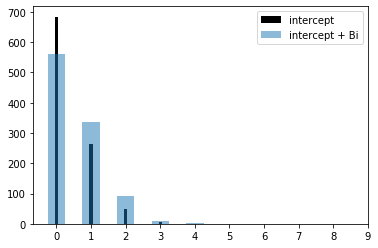
We can derive the model output using predict or the raw coefficients. Sampling the Poisson rate (lambda) illustrates the difference in predicted rates for the intercept and for a when a driver is male.
1
FreqPoisson.summary()
| Dep. Variable: | Claims | No. Observations: | 45183 |
|---|---|---|---|
| Model: | GLM | Df Residuals: | 45161 |
| Model Family: | Poisson | Df Model: | 21 |
| Link Function: | log | Scale: | 1.0000 |
| Method: | IRLS | Log-Likelihood: | -2541.7 |
| Date: | Wed, 14 Oct 2020 | Deviance: | 4135.6 |
| Time: | 21:43:22 | Pearson chi2: | 1.83e+05 |
| No. Iterations: | 22 | ||
| Covariance Type: | nonrobust |
| coef | std err | z | P>|z| | [0.025 | 0.975] | |
|---|---|---|---|---|---|---|
| Intercept | -0.9052 | 0.284 | -3.184 | 0.001 | -1.462 | -0.348 |
| Sex[T.M] | 0.3881 | 0.162 | 2.392 | 0.017 | 0.070 | 0.706 |
| Geog[T.2] | -0.6478 | 0.135 | -4.811 | 0.000 | -0.912 | -0.384 |
| Geog[T.3] | -0.9043 | 0.137 | -6.606 | 0.000 | -1.173 | -0.636 |
| Geog[T.4] | -1.3826 | 0.123 | -11.254 | 0.000 | -1.623 | -1.142 |
| Geog[T.5] | -1.5218 | 0.389 | -3.912 | 0.000 | -2.284 | -0.759 |
| Geog[T.6] | -1.4581 | 0.315 | -4.623 | 0.000 | -2.076 | -0.840 |
| Geog[T.7] | -22.0308 | 1.77e+04 | -0.001 | 0.999 | -3.47e+04 | 3.46e+04 |
| EV[T.2] | 0.0923 | 0.237 | 0.389 | 0.697 | -0.372 | 0.557 |
| EV[T.3] | -0.4219 | 0.199 | -2.115 | 0.034 | -0.813 | -0.031 |
| EV[T.4] | -0.3602 | 0.215 | -1.678 | 0.093 | -0.781 | 0.061 |
| EV[T.5] | -0.0334 | 0.204 | -0.164 | 0.870 | -0.433 | 0.367 |
| EV[T.6] | 0.4132 | 0.202 | 2.042 | 0.041 | 0.017 | 0.810 |
| EV[T.7] | 0.3316 | 0.483 | 0.687 | 0.492 | -0.614 | 1.278 |
| NCD[T.2] | -0.1441 | 0.181 | -0.795 | 0.426 | -0.499 | 0.211 |
| NCD[T.3] | 0.0184 | 0.192 | 0.096 | 0.923 | -0.357 | 0.394 |
| NCD[T.4] | 0.3047 | 0.184 | 1.660 | 0.097 | -0.055 | 0.664 |
| NCD[T.5] | -0.0535 | 0.215 | -0.249 | 0.804 | -0.475 | 0.368 |
| NCD[T.6] | 0.0967 | 0.206 | 0.470 | 0.639 | -0.307 | 0.501 |
| NCD[T.7] | 0.1835 | 0.137 | 1.334 | 0.182 | -0.086 | 0.453 |
| Age | -0.0580 | 0.004 | -13.633 | 0.000 | -0.066 | -0.050 |
| VehAge | -0.0762 | 0.008 | -9.781 | 0.000 | -0.091 | -0.061 |
1
2
Lambda intercept: 0.40
Lambda intercept + male: 0.60
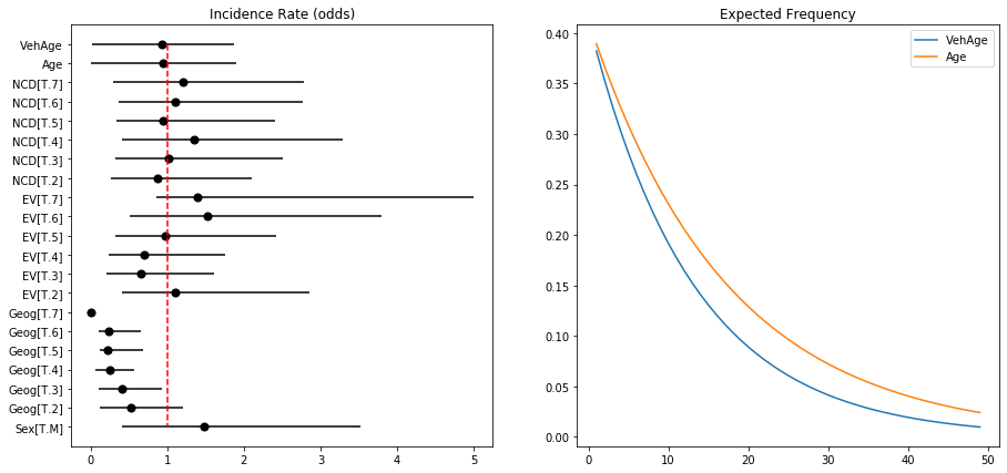
Negative binomial coefficients and incidence rate ratio
- https://stats.idre.ucla.edu/stata/dae/negative-binomial-regression/
- https://stats.stackexchange.com/questions/17006/interpretation-of-incidence-rate-ratios
- https://stats.stackexchange.com/questions/414752/how-to-interpret-incidence-rate-ratio
- https://www.cdc.gov/csels/dsepd/ss1978/lesson3/section5.html
1
print(FreqNegBin.summary())
1
2
3
4
5
6
7
8
9
10
11
12
13
14
15
16
17
18
19
20
21
22
23
24
25
26
27
28
29
30
31
32
33
34
35
36
37
                 Generalized Linear Model Regression Results
==============================================================================
Dep. Variable:                 Claims   No. Observations:                45183
Model:                            GLM   Df Residuals:                    45161
Model Family:        NegativeBinomial   Df Model:                           21
Link Function:                    log   Scale:                          1.0000
Method:                          IRLS   Log-Likelihood:                -2535.9
Date:                Wed, 14 Oct 2020   Deviance:                       3754.7
Time:                        21:43:23   Pearson chi2:                 1.82e+05
No. Iterations:                    21
Covariance Type:            nonrobust
==============================================================================
                 coef    std err          z      P>|z|      [0.025      0.975]
------------------------------------------------------------------------------
Intercept     -0.8851      0.288     -3.069      0.002      -1.450      -0.320
Sex[T.M]       0.3927      0.163      2.403      0.016       0.072       0.713
Geog[T.2]     -0.6545      0.137     -4.778      0.000      -0.923      -0.386
Geog[T.3]     -0.9104      0.139     -6.541      0.000      -1.183      -0.638
Geog[T.4]     -1.3888      0.125    -11.100      0.000      -1.634      -1.144
Geog[T.5]     -1.5350      0.391     -3.928      0.000      -2.301      -0.769
Geog[T.6]     -1.4693      0.317     -4.635      0.000      -2.091      -0.848
Geog[T.7]    -21.1594   1.13e+04     -0.002      0.999   -2.22e+04    2.22e+04
EV[T.2]        0.0957      0.240      0.399      0.690      -0.375       0.566
EV[T.3]       -0.4359      0.202     -2.155      0.031      -0.832      -0.039
EV[T.4]       -0.3671      0.217     -1.690      0.091      -0.793       0.059
EV[T.5]       -0.0319      0.207     -0.154      0.877      -0.437       0.373
EV[T.6]        0.4212      0.205      2.054      0.040       0.019       0.823
EV[T.7]        0.3309      0.486      0.681      0.496      -0.622       1.283
NCD[T.2]      -0.1456      0.183     -0.795      0.427      -0.505       0.214
NCD[T.3]       0.0171      0.194      0.089      0.929      -0.362       0.397
NCD[T.4]       0.2965      0.186      1.591      0.112      -0.069       0.662
NCD[T.5]      -0.0509      0.217     -0.234      0.815      -0.477       0.375
NCD[T.6]       0.1034      0.208      0.498      0.618      -0.303       0.510
NCD[T.7]       0.1871      0.139      1.343      0.179      -0.086       0.460
Age           -0.0581      0.004    -13.509      0.000      -0.067      -0.050
VehAge        -0.0766      0.008     -9.730      0.000      -0.092      -0.061
==============================================================================
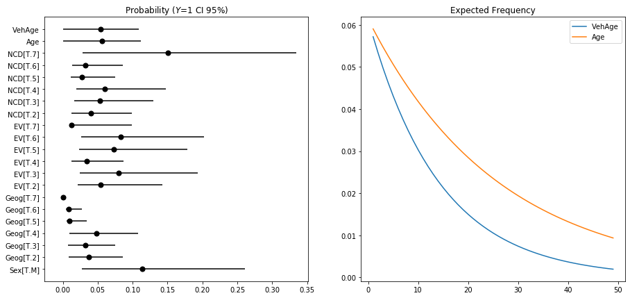
Binomial Model Coefficients and Logits Log-Odds, Odds and Probabilties
- https://sebastiansauer.github.io/convert_logit2prob/
1
print(FreqBinom.summary())
1
2
3
4
5
6
7
8
9
10
11
12
13
14
15
16
17
18
19
20
21
22
23
24
25
26
27
28
29
30
31
32
33
34
35
36
37
                 Generalized Linear Model Regression Results
==============================================================================
Dep. Variable:                  Claim   No. Observations:                45183
Model:                            GLM   Df Residuals:                 45690.29
Model Family:                Binomial   Df Model:                           21
Link Function:                  logit   Scale:                          1.0000
Method:                          IRLS   Log-Likelihood:                -3504.3
Date:                Wed, 14 Oct 2020   Deviance:                       7008.7
Time:                        21:43:23   Pearson chi2:                 4.72e+04
No. Iterations:                    24
Covariance Type:            nonrobust
==============================================================================
                 coef    std err          z      P>|z|      [0.025      0.975]
------------------------------------------------------------------------------
Intercept     -2.7911      0.289     -9.672      0.000      -3.357      -2.225
Sex[T.M]       0.7379      0.153      4.832      0.000       0.439       1.037
Geog[T.2]     -0.4605      0.141     -3.265      0.001      -0.737      -0.184
Geog[T.3]     -0.6028      0.140     -4.320      0.000      -0.876      -0.329
Geog[T.4]     -0.1851      0.111     -1.668      0.095      -0.403       0.032
Geog[T.5]     -1.8854      0.514     -3.667      0.000      -2.893      -0.878
Geog[T.6]     -2.0365      0.456     -4.469      0.000      -2.930      -1.143
Geog[T.7]    -21.7246   1.56e+04     -0.001      0.999   -3.07e+04    3.06e+04
EV[T.2]       -0.0613      0.261     -0.234      0.815      -0.574       0.451
EV[T.3]        0.3441      0.198      1.734      0.083      -0.045       0.733
EV[T.4]       -0.5492      0.226     -2.426      0.015      -0.993      -0.105
EV[T.5]        0.2531      0.204      1.238      0.216      -0.147       0.654
EV[T.6]        0.3888      0.207      1.882      0.060      -0.016       0.794
EV[T.7]       -1.5831      1.025     -1.544      0.123      -3.593       0.427
NCD[T.2]      -0.3731      0.198     -1.887      0.059      -0.761       0.015
NCD[T.3]      -0.0929      0.203     -0.458      0.647      -0.490       0.305
NCD[T.4]       0.0394      0.206      0.191      0.849      -0.365       0.443
NCD[T.5]      -0.7865      0.295     -2.671      0.008      -1.364      -0.209
NCD[T.6]      -0.6098      0.273     -2.230      0.026      -1.146      -0.074
NCD[T.7]       1.0612      0.123      8.654      0.000       0.821       1.302
Age           -0.0384      0.003    -11.086      0.000      -0.045      -0.032
VehAge        -0.0705      0.006    -11.589      0.000      -0.082      -0.059
==============================================================================
1
2
3
4
5
6
7
# Example conversions from logits to probabilities
const = FreqBinom.params[0]
odds = np.exp(const)
probability = odds / (1+odds)
print(f'Intercept: p = {probability:.3f}')
_ = np.exp(const+FreqBinom.params[1])/(1+(np.exp(const+FreqBinom.params[1])))
print(f'Intercept + Male: p = {_:.3f} ({_-probability:.3f})')
1
2
Intercept: p = 0.058
Intercept + Male: p = 0.114 (0.056)
Prediction
1
2
3
4
5
6
7
8
9
test['Fnb'] = FreqNegBin.predict(transform=True,exog=test,offset=np.log(test['PYrs']))
test['Fpo'] = FreqPoisson.predict(transform=True,exog=test,offset=np.log(test['PYrs']))
test['Fbi'] = FreqBinom.predict(transform=True,exog=test)

fig,axs = plt.subplots(1,3,figsize=(13,3.3),sharex=True,sharey=True)
sns.histplot(test['Fpo'],ax=axs[0],label='Poisson')
sns.histplot(test['Fnb'],ax=axs[1],label='NegBinomial')
sns.histplot(test['Fbi'],ax=axs[2],label='Binomial')
test.sample(5)
| Age | Sex | Geog | EV | VehAge | NCD | PYrs | Claims | Severity | Claim | SeverityAvg | Fnb | Fpo | Fbi | |
|---|---|---|---|---|---|---|---|---|---|---|---|---|---|---|
| 63584 | 69.0 | M | 4 | 1 | 5 | 3 | 0.361644 | 0 | 0.0 | 0 | 0.0 | 0.000694 | 0.000690 | 0.004815 |
| 2446 | 21.0 | M | 4 | 5 | 8 | 3 | 0.767123 | 0 | 0.0 | 0 | 0.0 | 0.018421 | 0.018198 | 0.030839 |
| 63505 | 69.0 | M | 1 | 1 | 11 | 7 | 0.665753 | 0 | 0.0 | 0 | 0.0 | 0.003833 | 0.003781 | 0.011952 |
| 7309 | 25.0 | M | 3 | 5 | 1 | 6 | 0.263014 | 0 | 0.0 | 0 | 0.0 | 0.015058 | 0.014718 | 0.017250 |
| 29573 | 42.0 | M | 6 | 6 | 7 | 7 | 0.257534 | 0 | 0.0 | 0 | 0.0 | 0.003391 | 0.003337 | 0.008624 |
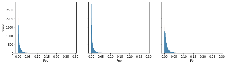
Looking at the model summaries, the histograms and results the of predicted values on the test, we see that each model weights covariates similarly and produces similar scores on the test data. Again note that the $Binomial$ model was only used to demonstrate its similarity in this case, but this may not hold for other data.
Claim Severity
1
2
3
4
5
6
7
# including PYrs as parameter commented out in glm()
expr = "SeverityAvg ~ Age + Sex + Geog + EV + VehAge + NCD"

### Estimate severity using GLM-gamma with default inverse-power link
SevGamma = smf.glm(formula=expr,
              data=train_severity,
              family=sm.families.Gamma(link=sm.families.links.inverse_power())).fit()
Ignore the warning for now we will come back to that.
After fitting a GLM-Gamma, how do we find the Gamma shape (a) and scale (b) parameters of predictions for Xi?
“Regression with the gamma model is going to use input variables Xi and coefficients to make a pre-diction about the mean of yi, but in actuality we are really focused on the scale parameter βi. This is so because we assume that αi is the same for all observations, and so variation from case to case in μi=βiα is due simply to variation in βi.” technical overview of gamma glm
- gamma handout
- Gamma Choice of link function
- exmaple finding scale in R
- generalized linear model - Dispersion parameter for Gamma family - Cross Validated
- Pdummy_xyhon: Calculating scale/dispersion of Gamma GLM using statsmodels
Alternatively you can infer gamma parameters from CI
- gamma.shape.glm: Estimate the Shape Parameter of the Gamma Distribution R MASS
- The identity link function does not respect the domain of the Gamma family? - Cross Validated
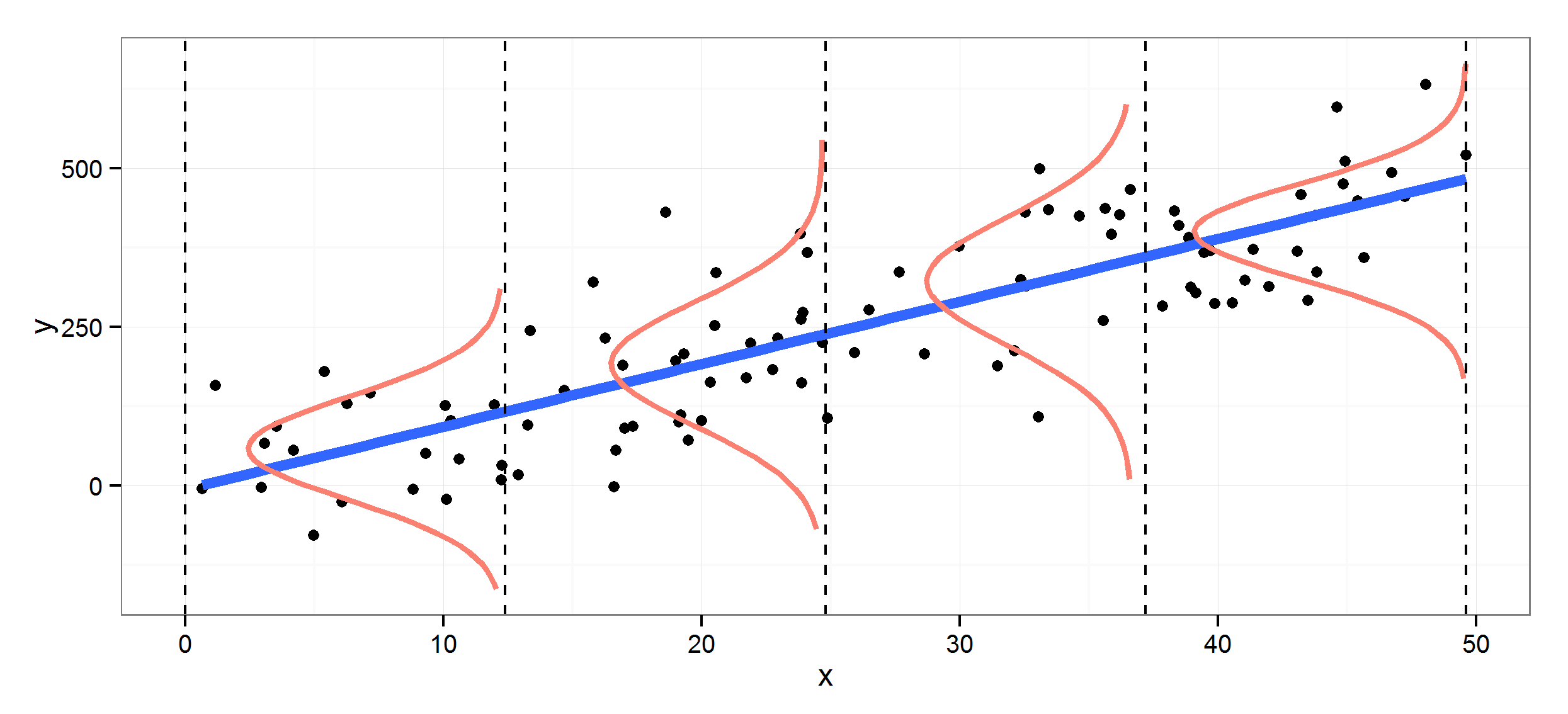
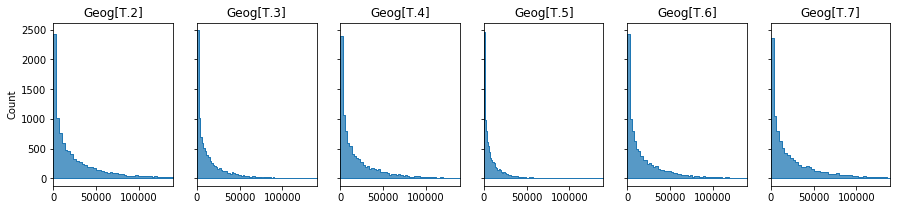
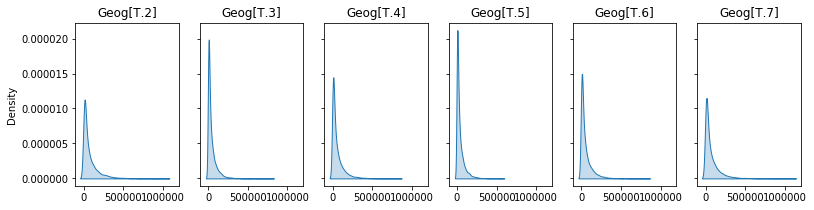
Below I illustrate the range of predicted severity values for the intercept and each level in Geography.
1
2
3
4
5
6
7
8
9
10
11
12
13
14
15
16
17
# shape is
shape = 1/SevGamma.scale
print(f'Shape: {shape:.2f}')

# intercept
constant,intercept = SevGamma.params[0],SevGamma.scale/SevGamma.params[0]
print(f'Intercept: {intercept:.0f}')

# predicted mean G(Yi) is exp(Bo + Bi*Xi..)
geogs = [(i,SevGamma.scale/(constant+c)) for i,c in zip(SevGamma.params.index,SevGamma.params) if 'Geog' in i]

# plot
fig,axs = plt.subplots(1,6,sharex=True,sharey=True,figsize=(15,3))
for ax,x in zip(axs.flatten(),geogs):
    sns.histplot(np.random.gamma(shape=shape,scale=x[1],size=10000),stat="count",element="step",ax=ax,)
    ax.set_title(x[0])
    ax.set_xlim(0,14e4)
1
2
Shape: 0.54
Intercept: 52203
The GLM-Gamma model gives us a prediction of the average severity of a claim should one occur.
1
2
test_severity['Giv'] = SevGamma.predict(transform=True,exog=test_severity)
test_severity[:3]
| Age | Sex | Geog | EV | VehAge | NCD | PYrs | Claims | Severity | Claim | SeverityAvg | Giv | |
|---|---|---|---|---|---|---|---|---|---|---|---|---|
| 35445 | 45.0 | M | 4 | 6 | 2 | 7 | 4.920548 | 1 | 2480.0 | 1 | 2480.0 | 28728.757724 |
| 9653 | 26.0 | M | 6 | 6 | 9 | 5 | 0.589041 | 1 | 46000.0 | 1 | 46000.0 | 21782.480267 |
| 2039 | 21.0 | M | 2 | 2 | 19 | 1 | 0.432877 | 1 | 11110.0 | 1 | 11110.0 | 11537.649676 |
Now, remember the error we got using the inverse-power link function. The warning is fairly self explanatory “the inverse_power link function does not respect the domain of the Gamma family”. Oddly this is a design feature of Statsmodels at the time of writing. Rather it is better to use the log link function to ensure all predicted values are > 0.
GLM-Gamma log link
1
2
3
4
5
6
7
# formula
expr = "SeverityAvg ~ Age + Sex + Geog + EV + VehAge + NCD"

### Estimate severity using GLM-gamma with default log link
SevGamma = smf.glm(formula=expr,
                   data=train_severity,
                   family=sm.families.Gamma(link=sm.families.links.log())).fit()
1
2
3
4
5
6
7
8
9
10
11
12
13
14
15
16
17
18
19
20
21
22
23
24
25
# dispersion aka rate
dispersion = SevGamma.scale
print(f'Dispersion: {dispersion:.4f}')

# shape is 1/dispersion
shape = 1/dispersion
print(f'Shape: {shape:.4f}')

# intercept
constant,intercept = SevGamma.params[0],np.exp(SevGamma.params[0])
print(f'Intercept: {intercept:.2f}')

# predicted mean G(Yi) is exp(Bo + Bi*Xi..)
# tuple(name,Yi,scale)
geogs = [(i,
          np.exp(constant+c),
          np.exp(constant+c)*dispersion)
         for i,c in zip(SevGamma.params.index,SevGamma.params) if 'Geog' in i]

# plot
fig,axs = plt.subplots(1,6,sharex=True,sharey=True,figsize=(13,3))

for ax,x in zip(axs.flatten(),geogs):
    sns.kdeplot(np.random.gamma(shape=shape,scale=x[2],size=10000),shade=True,ax=ax,)
    ax.set_title(x[0])
1
2
3
Dispersion: 2.0528
Shape: 0.4872
Intercept: 69330.81
Statsmodels uses patsy design matrices behind the scenes. We can apply the design matrix to calculate the distribution parameters for both the frequency and severity models, and for any data set. Train, test, synthetic data and portfolios. You name it.
This is an incredibly powerfull approach as it enables the development of highly parameterised Monte Carlo and risk simulation models.I will walk the steps using pandas dataframes so that it is clear:
1
2
3
4
5
6
7
8
9
10
11
12
13
14
15
16
17
# 1. Define a dummy model for your data and using the same formula and settings defined earlier.
dummy_ = smf.glm(formula=expr,data=test_severity,family=sm.families.Gamma(link=sm.families.links.log()))

# 2. we can then access the desing matrix.
# Which is simply the data values, but also handling the intercept and reference categories.
a = pd.DataFrame(dummy_.data.exog,columns=dummy_.data.param_names)

# 3. Retrieve and transpose the trained model coefficients
b = pd.DataFrame(SevGamma.params).T

# 4. And multiply together
# but this only works if indexes are equal
c = a.multiply(b,axis=0)

# 5. It is much cleaner to use arrays.
# et voila
c = pd.DataFrame(dummy_.data.exog * SevGamma.params.values,columns=dummy_.data.param_names)
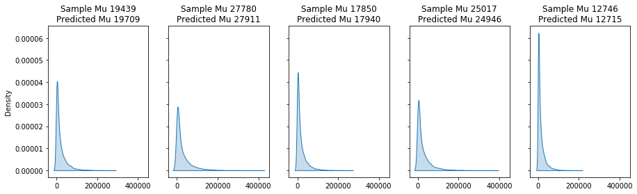
We can then use the coefficients to estimate and plot the values and samples of each row, or the entire dataset.
1
2
3
4
5
6
7
8
9
10
11
dispersion = SevGamma.scale
shape = 1/dispersion

num=5
fig,axs = plt.subplots(1,num,figsize=(15,4),sharex=True,sharey=True)

for i,pred,ax in zip(c.index[:num],SevGamma.predict(test_severity)[:num],axs.flatten()):
    scale = np.exp(c.loc[[i]].sum(axis=1))*dispersion
    sample = np.random.gamma(shape=shape,scale=scale,size=10000)
    sns.kdeplot(sample,label=i,ax=ax,shade=True)
    ax.set_title(f'Sample Mu {sample.mean():.0f}\nPredicted Mu {pred:.0f}',fontsize=12)
Putting it all together: Frequency-Severity model
Portfolio price
Given that this is motor insurance, lets assume a thin margin for %0.05
1
2
3
4
5
6
7
8
9
10
11
12
13
14
# make a dummy portfolio and make predictions
portfolio = test.reset_index(drop=True).copy()
portfolio['annual_frq'] = FreqBinom.predict(portfolio)
portfolio['expected_sev'] = SevGamma.predict(portfolio)

# expected annual loss
portfolio['annual_exp_loss'] = portfolio['annual_frq'] * portfolio['expected_sev']

# set pricing ratio
tolerable_loss = 0.05
pricing_ratio = 1.0-tolerable_loss
portfolio['annual_tech_premium'] = portfolio['annual_exp_loss']/pricing_ratio
portfolio['result'] = portfolio['annual_tech_premium'] - portfolio['Severity']
portfolio.iloc[:3,-4:]
| expected_sev | annual_exp_loss | annual_tech_premium | result | |
|---|---|---|---|---|
| 0 | 27818.169806 | 277.316838 | 291.912461 | 291.912461 |
| 1 | 21753.203517 | 300.218299 | 316.019262 | 316.019262 |
| 2 | 18524.970346 | 298.920877 | 314.653555 | 314.653555 |
This summary illustrates the:
- observed Claims and Losses (Severity)
- the predicted frq, losses, and expected-losses
- the technical premium
- the profit loss result (calculated on full Severity rather than SeverityAvg)
| Claim | Severity | annual_frq | expected_sev | annual_exp_loss | annual_tech_premium | result | |
|---|---|---|---|---|---|---|---|
| Summary | 201.0 | 5377478.0 | 249.038867 | 4.054346e+08 | 5.764319e+06 | 6.067705e+06 | 690226.503245 |
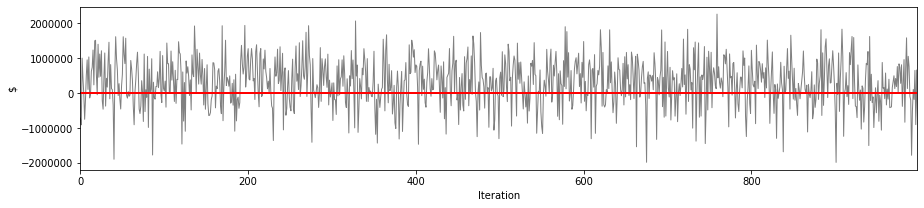
Now we can build a Monte Carlo simulation to:
- provide a more robust estimate of our expected profit / loss
- sample the parameter space to gauge the variance and uncertainty in our model and assumptions
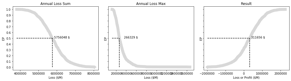
- calculate metrics for the AAL, AEP, and AXS loss and return
1
2
3
4
5
6
7
8
9
10
11
12
13
14
15
16
17
18
19
20
21
22
# simulate portfolio
simulation = dict()
frq = list()
sev = list()
N=999

for it in range(N):
    print(f"{it}/{N}",end='\r')

    frq.append(np.random.binomial(n=1,p=portfolio['annual_frq']))
    sev.append(np.random.gamma(shape=portfolio['gamma_shape'],scale=portfolio['gamma_scale']))

# calculate Frq * Sev
frq_sev = np.array(frq)*np.array(sev)
# summarise the simulations
simulation['sim'] = pd.DataFrame({'iteration':range(N),
                                  'claim_num':np.array(frq).sum(axis=1),# num claims
                                  'loss_min':np.array(frq_sev).min(axis=1), # min claim
                                  'loss_sum':np.array(frq_sev).sum(axis=1), # total
                                  'loss_max':np.array(frq_sev).max(axis=1), # max claim
                                  'loss_avg':np.array(frq_sev).mean(axis=1)
                              })
1
998/999
Calculate the Annual Exceedence Probability
- https://sciencing.com/calculate-exceedance-probability-5365868.html
- https://serc.carleton.edu/quantskills/methods/quantlit/RInt.html
- https://www.earthdatascience.org/courses/use-data-open-source-python/use-time-series-data-in-python/floods-return-period-and-probability/
1
2
3
4
5
6
7
8
9
10
11
12
13
14
15
16
17
18
def exceedance_prob(df,feature,ascending=False):
    data = df.copy()
    data['value'] = data[feature]
    data[f'Rank'] = data['value'].rank(ascending=ascending,method='dense')
    data[f'RI'] = (len(data)+1.0)/data[f'Rank']
    data[f'EP'] = 1.0/data[f'RI']
    data.sort_values([f'value'],ascending=ascending,inplace=True)
    data.reset_index(drop=True,inplace=True)
    return data

# profit loss based on technical premium
simulation['sim']['technical_premium'] = portfolio['annual_tech_premium'].sum()
simulation['sim']['result'] = (simulation['sim']['technical_premium'] - simulation['sim']['loss_sum'])

# recurrence intervals of each measure
simulation['loss_sum'] = exceedance_prob(simulation['sim'],'loss_sum')
simulation['loss_max'] = exceedance_prob(simulation['sim'],'loss_max')
simulation['result'] = exceedance_prob(simulation['sim'],'result',ascending=True)
This illustrates the profit and loss scenarios for our pricing strategy across $N$ iterations.
And more intuitive EP curves.