
In this post I will show how Bayesian inference is applied to train a model and make predictions on out-of-sample test data. For this, we will build two models using a case study of predicting student grades on a classical dataset. The first model is a classic frequentist normally distributed regression General Linear Model (GLM). While the second is, again A normal GLM, but built using the Bayesian inference method.
Case Study: predicting student grades
The objective is to develop a model that can predict student grades given several input factors about each student. The publicly available UCI dataset contains grades and factors for 649 students taking a Portuguese language course. #
Dependent variable or “Target”
- “G3” is the student’s final grade for Portuguese (numeric: from 0 to 20, output target)
Independent variables or “Features”
A subset of numeric and categorical features is used to build the initial model:
- “age” student age from 15 to 22
- “internet” student has internet access at home (binary: yes or no)
- “failures” is the number of past class failures (cat: n if 1<=n<3, else 4)
- “higher” wants to take higher education (binary: yes or no)
- “Medu” mother’s education (cat: 0 - none, 1 - primary education (4th grade), 2 5th to 9th grade, 3 secondary education or 4 higher education)
- "”Fedu father’s education (cat: 0 - none, 1 - primary education (4th grade), 2 5th to 9th grade, 3 secondary education or 4 higher education)
- “studytime” weekly study time (cat: 1 - <2 hours, 2 - 2 to 5 hours, 3 - 5 to 10 hours, or 4 - >10 hours)
- “absences” number of school absences (numeric: from 0 to 93)
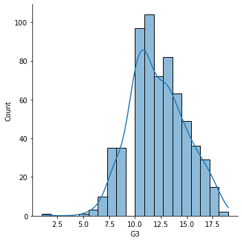
The final dataset looks like this and here is the distribution of acheived student grades for Portuguese.
| internet | higher | age | absences | failures | Medu | Fedu | studytime | G3 | |
|---|---|---|---|---|---|---|---|---|---|
| 0 | 0 | 1 | 18 | 4 | 0 | 4 | 4 | 2 | 11 |
1
sns.displot(data=df,x='G3',kde=True);
GLM: frequentist model
First, I will build a regular GLM using statsmodels to illustrate the frequentist approach.
There are two binary categorical features for Internet usage and Higher education. Age is a numerical feature. The remaining features are numerical values that have been cut into ordinal categories. Practitioners may treat these differently depending on the model objective and nature of the feature. Here I will treat them as numerical within range 0 to max(feature) range. In statsmodels we can use patsy design matrices and formula to specify how we want to treat each variable. For instance, for categoricals, we can use C(Internet, Treatment(0)) to encode Internet as a categorical variable with the reference level set to (0).
1
2
3
4
5
6
7
8
# model grade data
formula = [f"{f}" if f not in categoricals else f"C({f})" for f in features]
formula = f'{target[0]} ~ ' + ' + '.join(formula)
glm_ = smf.glm(formula=formula,
              data=df,
              family=sm.families.Gaussian())
glm = glm_.fit()
glm.summary()
| Dep. Variable: | G3 | No. Observations: | 634 |
|---|---|---|---|
| Model: | GLM | Df Residuals: | 625 |
| Model Family: | Gaussian | Df Model: | 8 |
| Link Function: | identity | Scale: | 5.1895 |
| Method: | IRLS | Log-Likelihood: | -1417.1 |
| Date: | Fri, 12 Mar 2021 | Deviance: | 3243.4 |
| Time: | 13:39:15 | Pearson chi2: | 3.24e+03 |
| No. Iterations: | 3 | ||
| Covariance Type: | nonrobust |
| coef | std err | z | P>|z| | [0.025 | 0.975] | |
|---|---|---|---|---|---|---|
| Intercept | 3.6741 | 1.430 | 2.570 | 0.010 | 0.872 | 6.476 |
| C(internet)[T.1] | 0.2882 | 0.225 | 1.282 | 0.200 | -0.152 | 0.729 |
| C(higher)[T.1] | 1.8413 | 0.328 | 5.622 | 0.000 | 1.199 | 2.483 |
| age | 0.3185 | 0.081 | 3.945 | 0.000 | 0.160 | 0.477 |
| absences | -0.0739 | 0.020 | -3.674 | 0.000 | -0.113 | -0.034 |
| failures | -1.4217 | 0.170 | -8.339 | 0.000 | -1.756 | -1.088 |
| Medu | 0.3847 | 0.108 | 3.567 | 0.000 | 0.173 | 0.596 |
| Fedu | 0.0332 | 0.108 | 0.306 | 0.760 | -0.179 | 0.246 |
| studytime | 0.4307 | 0.112 | 3.839 | 0.000 | 0.211 | 0.651 |
Some quick observations on the above. Most features have a statistically significant linear relaitonship with grade with the exception of Fathers education. The sign of the regression coefficients also hold with our logic. More absensences and failures is shown to have a negative influence on predicted grade. Whereas studytime and desire to go on to higher education having positive influence on predicted grade.
Below we see there is an outlier in the data.

PyMC3 GLM: Bayesian model
Now let’s re-build our model using PyMC3. As described in this blog post PyMC3 has its own glm.from_formula() function that behaves similar to statsmodels. It even accepts the same patsy formula.
1
2
3
4
5
6
7
8
9
10
11
12
13
14
import pymc3 as pm
import arviz as avz

# note we can re-use our formula
print(formula)

bglm = pm.Model()
with bglm:
    # Normally distributed priors
    family = pm.glm.families.Normal()
    # create the model
    pm.GLM.from_formula(formula,data=df,family=family)
    # sample
    trace = pm.sample(1000,return_inferencedata=True)
1
2
3
4
5
6
G3 ~ C(internet) + C(higher) + age + absences + failures + Medu + Fedu + studytime

Auto-assigning NUTS sampler...
Initializing NUTS using jitter+adapt_diag...
Multiprocess sampling (4 chains in 4 jobs)
NUTS: [sd, studytime, Fedu, Medu, failures, absences, age, C(higher)[T.1], C(internet)[T.1], Intercept]
Once the model has run we can examine the model posterior distribution samples. This is akin to viewing the model.summary() of a regular GLM as above. In this Bayesian model summary table the mean is the coefficient estimate from the posterior distribution. Here we see the posterior distribution of the model intercept is around 4.9. Indicating a student is expected to attain at least a grade of 4.9 irrespective of what we know about them.
1
2
summary = avz.summary(trace)
summary[:5]
| mean | sd | hdi_3% | hdi_97% | mcse_mean | mcse_sd | ess_bulk | ess_tail | r_hat | |
|---|---|---|---|---|---|---|---|---|---|
| Intercept | 3.724 | 1.421 | 0.997 | 6.260 | 0.026 | 0.019 | 2972.0 | 2599.0 | 1.0 |
| C(internet)[T.1] | 0.287 | 0.221 | -0.126 | 0.706 | 0.003 | 0.003 | 4183.0 | 2580.0 | 1.0 |
| C(higher)[T.1] | 1.836 | 0.332 | 1.188 | 2.450 | 0.005 | 0.004 | 4244.0 | 2697.0 | 1.0 |
| age | 0.315 | 0.080 | 0.167 | 0.463 | 0.001 | 0.001 | 2950.0 | 2281.0 | 1.0 |
| absences | -0.074 | 0.021 | -0.114 | -0.035 | 0.000 | 0.000 | 5348.0 | 2799.0 | 1.0 |
Rather than p-values we have highest posterior density “hpd”. The 3-97% hpd fields and value range indicates the credible interval for the true value of our parameter. As for classical models if this range crosses 0, from negative affect to positive affect, then perhaps the data signal is too weak to draw conclusions for this variable. This is the case for Internet usage - darnit Covid19.
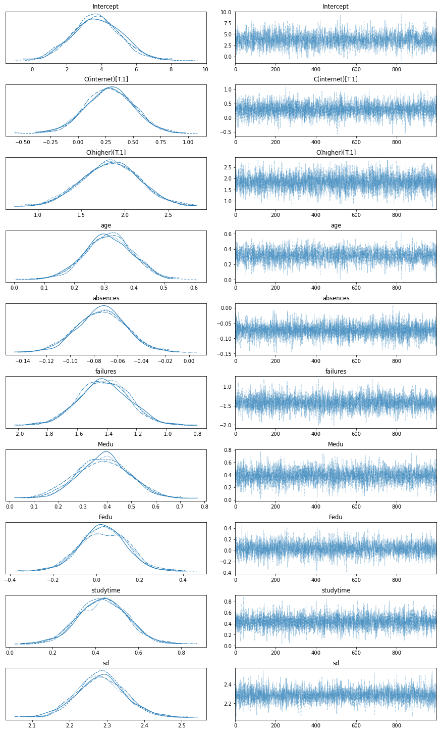
The posterior distributions can also be viewed as traceplots.
1
avz.plot_trace(trace)
Interpret Variable affect on Predicted Grade
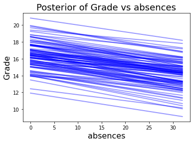
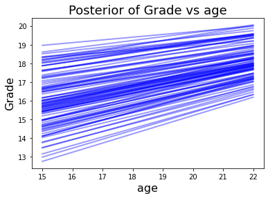
With the sampling complete. We can explore how each feature affects and contributes to predicted grade. I found this model_affect() function in this Gist for PyMC3.
Again, the number of absences has a negative affect on epected grade. Increasing age has a positive affect.
1
2
3
X = pd.DataFrame(data=glm_.data.exog,columns=glm_.data.param_names) # dmatrix
model_affect('absences',trace,X)
model_affect('age',trace,X)
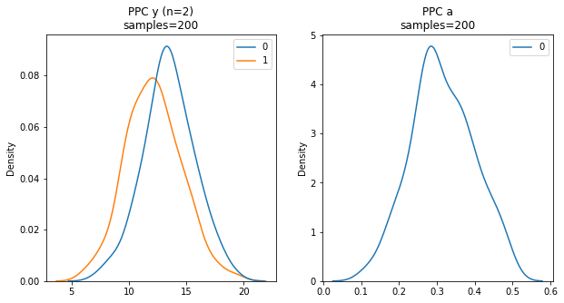
Posterior Predictive Checks
Posterior predictive checks (PPC’s) are conducted to validate that the Bayesian model has captured the true distribution of the underlying data. Alternatively, PPC’s are used to evaluate how the true data distribution compares to the distribution of data generates by the Bayesian model. . As per the PyMC3 documentation, PPC’s are also a crucial part of the Bayesian modeling workflow. PPC’s have two main benefits:
- They allow you to check whether you are indeed incorporating scientific knowledge into your model – in short, they help you check how credible your assumptions before seeing the data are.
- They can help sampling considerably, especially for generalized linear models, where the outcome space and the parameter space diverge because of the link function.
Below, PPC is used to sample the Y outcome of our model 200 times (left). Similar to the above trace plots, PPC can also provide a sampling of model parameters such as Age (right).
Predictions on Out-Of-Sample data
Now that the model is trained and fitted on the data and we have inspected variable affects we can use the model to make predictions on out-of-sample observations and test cases. In contrast to other modeling approaches and packages, such as statsmodels and scikit-learn, it is not as straight forward as simply calling model.predict(Xdata). In PyMC3 I have discovered several strategies for applying models to out-of-sample data.
method 1: the mean coefficient model
We can use the MCMC trace to obtain a sample mean of each model coefficient and apply this to reconstruct a typical GLM formula. Remember we used statsmodels-patsy formulation to encode our categorical variables, well we can again use patsy to construct a helper.
The benefit to this approach is its ease and simplicity. The downside is that we are now omitting and missing out on a chunk of that MCMC sampling for the confidence and uncertainty in our data that we obtained by taking a Bayes approach in the first place.
1
2
3
4
5
6
7
8
9
10
11
12
13
14
15
16
17
18
19
# mean model coefficients
mean_model = summary[['mean']].T.reset_index(drop=True)

# create a  design matrix of exog data values
# same as for GLM's
X = pd.DataFrame(data=glm_.data.exog,columns=glm_.data.param_names)

# add columns for the standard deviations output from the bayesian fit
for x in mean_model.columns:
    if x not in X.columns:
        X[x] = 1

# multiply and work out mu predictions
coefs = X * mean_model.values
pred_mu = coefs.iloc[:,:-1].sum(axis=1)[:]
pred_sd = coefs['sd']
print('Predictions:')
n = 5
for m,s in zip(pred_mu[:n],pred_sd[:n]): print(f"\tMu:{m:.2f} Sd:{s:.2f}")
1
2
3
4
5
6
Predictions:
	Mu:13.47 Sd:2.29
	Mu:12.34 Sd:2.29
	Mu:11.41 Sd:2.29
	Mu:13.48 Sd:2.29
	Mu:12.72 Sd:2.29
NOTE:: There is an issue using Jupyter, pymc3.GLM and Theano. At the time of writing this is where things with
pm.GLM.from_formula()start to break down using Jupyter. The following two methods are recommended in the PyMC3 documentation. However, both generate the following Theano error when used in conjunction withGLM.from_formula()on Jupyter.ERROR! Session/line number was not unique in database. History logging moved to new session 11This seems to be an issue with the way GLM.from_formula() uses patsy and interacts with Theano in Jupyter Notebooks.
source code
question on SO
I have not tested running either of the following methods using a .py script but it seems reasonable that the following methods would work outside Jupyter.
method 2: using Theano shared variable
Given the above, for now we will lose GLM.from_formula() and reconstruct the model in standard PyMC3 form and using both: patsy to generate a design matrix, and Theano to create a shared X variable. To keep things short I have simplified my Betas using shape(n). This will degrade model tuning performance as all priors are set at the uniform initial value and it may lead to some zero errors e.g see here. In practice, you should set the Beta’s individually using informative priors.
1
2
3
4
5
6
7
8
9
10
11
12
13
14
15
16
17
18
19
20
21
22
import patsy
from theano import shared

design = patsy.dmatrices(formula_like=formula,data=df,return_type='dataframe')
# design[1].design_info

train,test = df[:500],df[500:]
trainx = patsy.build_design_matrices([design[1].design_info],train,return_type="dataframe")[0]
testx = patsy.build_design_matrices([design[1].design_info],test,return_type="dataframe")[0]

# Shared theano variable for modeling
# must be np.array()
modelx = shared(np.array(trainx))

bglm = pm.Model()
with bglm:
    alpha = pm.Normal('alpha', mu=4, sd=10)
    betas = pm.Normal('beta', mu=1, sd=6, shape=8)
    sigma = pm.HalfNormal('sigma', sd=1)a)
    mu = alpha + pm.math.dot(betas, modelx.T)
    likelihood = pm.Normal('y', mu=mu, sd=sigma, observed=trainy)
    trace = pm.sample(1000,init="adapt_diag",return_inferencedata=True)
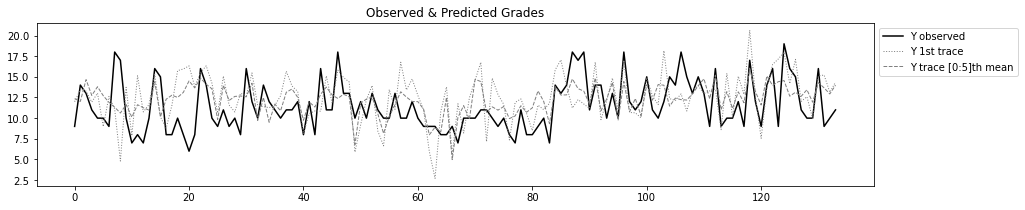
Now we can update our shared X variable with the test set and use the model to make predictions. The prediction here really means sampling the posterior distributions of each coefficient on the test set observations.
We can specify the number of sampling rounds to perform and visualise individual samples and aggregates of samples.
1
2
3
4
5
6
7
8
9
10
11
12
13
14
samples = 50

# Update model X and make Prediction
modelx.set_value(np.array(testx)) # update X data
ppc = pm.sample_posterior_predictive(trace, model=bglm, samples=samples,random_seed=6)
print(ppc['y'].shape)

n = 5
plt.figure(figsize=(15,3))
plt.title('Observed & Predicted Grades')
plt.plot(test.reset_index()['G3'],'k-',label='Y observed')
plt.plot(ppc['y'][0,:],lw=1,linestyle=':',c='grey',label='Y 1st trace')
plt.plot(ppc['y'][:n,:].mean(axis=0),lw=1,linestyle='--',c='grey',label=f'Y trace [0:{n}]th mean')
plt.legend(bbox_to_anchor=(1,1));
method 3: shared X variable
This method is very similar above but instead using the pm.Data() to hold our X data in train and test rounds. Functionally this is cleaner as we don’t need to import and use Theano shared() explicitly.
1
2
3
4
5
6
7
8
9
10
11
12
13
14
15
bglm = pm.Model()
with bglm:
    alpha = pm.Normal('alpha', mu=4, sd=10)
    betas = pm.Normal('beta', mu=1, sd=6, shape=8)
    sigma = pm.HalfNormal('sigma', sd=1)
    xdata = pm.Data("pred", trainx.T)
    mu = alpha + pm.math.dot(betas, xdata)
    likelihood = pm.Normal('y', mu=mu, sd=sigma, observed=trainy)
    trace = pm.sample(1000,init="adapt_diag",return_inferencedata=True)

# Update X values and predict outcomes and probabilities
with bglm:
    pm.set_data({"pred": testx.T})
    posterior_predictive = pm.sample_posterior_predictive(trace, var_names=["y"], samples=600)
    model_preds = posterior_predictive["y"]
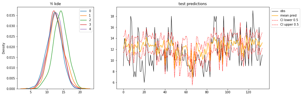
Again, let’s increase the number of samples visualise the:
- posterior distribution of predictions for each observation in the OOS test data (left)
- and the Observed, Mean, Credible-Interval or “Highest Density Interval” using arviz
hdi().
1
2
3
4
5
6
7
8
9
10
11
12
13
14
15
16
17
18
19
from matplotlib.gridspec import GridSpec

fig=plt.figure(figsize=(15,5))
gs=GridSpec(nrows=1,ncols=2,width_ratios=[1,2]) # 2 rows, 3 columns

ax0 = fig.add_subplot(gs[0])
ax0.set_title("Yi kde")
sns.kdeplot(data=pd.DataFrame(model_preds[:,:5]),ax=ax0)

ax1 = fig.add_subplot(gs[1])
ax1.set_title("test predictions")
ax1.plot(test.reset_index(drop=True)['G3'],'k-',lw=1,label='obs')
ax1.plot(model_preds.mean(0),c='orange',label='mean pred')

alpha = 1-0.5
ax1.plot(avz.hdi(model_preds,alpha)[:,0],ls='--',lw=1,c='red',label=f'CI lower {alpha}')
ax1.plot(avz.hdi(model_preds,alpha)[:,1],ls='--',lw=1,c='red',label=f'CI upper {alpha}')

ax1.legend(bbox_to_anchor=(1,1));
Conclusion
This post demonstrates how to develop a Bayesian inference General Linear Model. A case study for modeling student grades was used to demonstrate a classical frequentist approach in statsmodels and with a Bayes’s approach in PyMC3 with several implementations on predicting out of sample data.